TL;DR
I select a linear model with slope and intercept parameters to describe the growth dynamics of the EU industry production index of each country.
Long Description
Inspired by line plots of the EU industry production index time series that were previously normalized by the EU average time series, I choose to model the individual countries’ time series as linear in the available period covering the years 2000–2017. Concretely, I will use the linear model from the scikit-learn package and prepare the data accordingly by transforming the time axis. As a rough means to evaluate the robustness of the slope parameter, I decide to compare it to the difference of the last and first data points divided by the number of years.
Table of contents
Project Background
In the previous project, I have divided the EU industry production index time series for each country by the EU average to obtain a set of time series that are largely independent of the common development.
I now want to distill single numbers from the time series that capture the growth behavior for each country and allow an easy comparison. For that purpose, I am looking for a parameterized model that describes the long-term trends of the time series.
Choosing a model
Inspecting the data
I first read in the normalized EU industry production index time series:
import pandas as pd
df = pd.read_pickle('EU_industry_production_dataframe_normalized_2000-2017.pkl')
df.info()
print(df.head())
<class 'pandas.core.frame.DataFrame'>
MultiIndex: 7632 entries, (2000-01-01 00:00:00, AT) to (2017-08-01 00:00:00, UK)
Data columns (total 3 columns):
production_index         7412 non-null float64
flags                    7632 non-null category
production_index_norm    7404 non-null float64
dtypes: category(1), float64(2)
memory usage: 155.5+ KB

                         production_index flags  production_index_norm
time       country_code
2000-01-01 AT                        73.0                     0.763119
           BA                         NaN                          NaN
           BE                        63.1                     0.659628
           BG                        61.1                     0.638720
           CY                       103.0                     1.076730
To get a better view at the individual time series, I split the 36 curves into two plots. I select first only the first half and then only the second half of the country columns using the iloc locator:
import matplotlib.pyplot as plt
import numpy as np

################# First figure
fig, ax = plt.subplots()        # Create figure and axes objects

# Reset line properties to avoid ambiguity between different lines:
ax.set_prop_cycle(color=plt.cm.nipy_spectral(np.linspace(0,1,36)),linestyle=['-','--',':']*12)

# Create the plot:
ax = df['production_index_norm'].unstack(level=1).iloc[:,0:18].plot(ax=ax)
plt.xlabel('Year')
plt.ylabel('Production index [relative to EU28 avg.]')
ax.legend(ncol=6, fontsize=7)   # Adjust shape (four columns instead of one) and font size of legend
plt.show()

################# Second figure
fig, ax = plt.subplots()        # Create figure and axes objects

# Reset line properties to avoid ambiguity between different lines:
ax.set_prop_cycle(color=plt.cm.nipy_spectral(np.linspace(0.5,1,18)),linestyle=['-','--',':']*6)

# Create the plot:
ax = df['production_index_norm'].unstack(level=1).iloc[:,18:].plot(ax=ax)
plt.xlabel('Year')
plt.ylabel('Production index [relative to EU28 avg.]')
ax.legend(ncol=6, fontsize=7)   # Adjust shape (four columns instead of one) and font size of legend
plt.show()
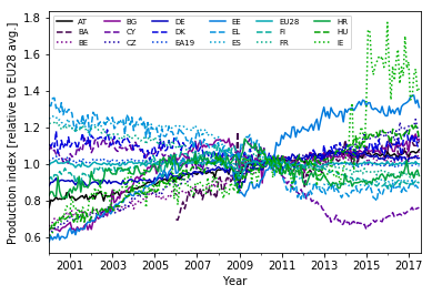
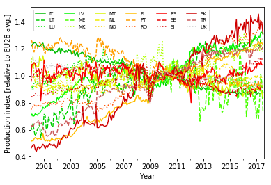
Though there are a few curves that show more complex long-term dynamics (e.g., Cyprus, CY), the vast majority can be described as roughly linear plus some short- to mid-scale fluctuations.
Linear approximation
This motivates a linear approximation of the time series. In such a simple model, y = m * x + b, the production index (y) depends on the time (x) and on two parameters: m gives the slope of the line and is thus a measure of the growth that I am looking for, b is the production index value at time zero (the intercept).
Time zero is a bit unpractical though when using the calendar year to express time. A more natural approach would be to count years from the reference point of the dataset, that is the year 2010.
How do I get a linear approximation of the time series? What I want is to find those values for m and b that minimize the sum of squared distances between the line and the real production index at each time (sum of squared residuals). This process is called linear regression.
Since y does only depend on one variable (x) in this case, I could use the numpy method polyfit() for this task.
In the spirit of a more general answer that would also work for more complex datasets (y depending on many variables), I opt to use the linear regression method in the scikit-learn package though.
Model evaluation
The quality of the model could be evaluated in different ways. One measure is the sum of the squared residuals, which acts as a cost function. It can be used as a basis to test if the time series is linear plus random noise. As I already know from the plots that there are also more complex mid-scale features, the benefits of such a test are limited though.
The model’s predictive power or consistency over time could be assessed by splitting the dataset in two (or more) parts. However, the time series is quite short.
Instead I will use a simple robustness check of the slopes from linear regression: I will also obtain m from a simple difference of the production index between the last and first data points in the time series. Dividing this difference by the number of years should give an alternative measure of m
Data preparation
Before performing the linear regression in the next project, I make the transformation of the time axis and unstack the “country_code” index level:
# Unstack country_code index into columns:
df_forregression = df['production_index_norm'].unstack(level=1).copy()

# Reset DatetimeIndex to FloatIndex (counting years from 2010):
df_forregression.set_index((df_forregression.index - pd.Timestamp('2010-01-01')) / pd.Timedelta(365.25, unit='d'), inplace=True)
print(df_forregression.info())
print(df_forregression.head())
Float64Index: 212 entries, -10.0013689254 to 7.58110882957
Data columns (total 36 columns):
AT 211 non-null float64
BA 139 non-null float64
BE 211 non-null float64
BG 211 non-null float64
CY 211 non-null float64
CZ 211 non-null float64
DE 211 non-null float64
DK 211 non-null float64
EA19 211 non-null float64
EE 211 non-null float64
EL 211 non-null float64
ES 211 non-null float64
EU28 211 non-null float64
FI 211 non-null float64
FR 211 non-null float64
HR 211 non-null float64
HU 211 non-null float64
IE 211 non-null float64
IT 211 non-null float64
LT 211 non-null float64
LU 211 non-null float64
LV 211 non-null float64
ME 91 non-null float64
MK 211 non-null float64
MT 211 non-null float64
NL 211 non-null float64
NO 211 non-null float64
PL 211 non-null float64
PT 211 non-null float64
RO 211 non-null float64
RS 211 non-null float64
SE 211 non-null float64
SI 211 non-null float64
SK 211 non-null float64
TR 211 non-null float64
UK 211 non-null float64
dtypes: float64(36)
memory usage: 61.3 KB
None
country_code AT BA BE BG CY CZ DE \
time
-10.001369 0.763119 NaN 0.659628 0.638720 1.076730 0.609450 0.882291
-9.916496 0.804837 NaN 0.675563 0.650542 1.094662 0.628649 0.900751
-9.837098 0.799001 NaN 0.682480 0.650229 1.071577 0.636704 0.900957
-9.752225 0.806887 NaN 0.703174 0.646132 1.076540 0.650280 0.909562
-9.670089 0.819436 NaN 0.705168 0.643401 1.054149 0.660902 0.923410
country_code DK EA19 EE … NO PL \
time …
-10.001369 1.108091 1.015053 0.577044 … 0.993101 0.510140
-9.916496 1.097790 1.027940 0.606756 … 0.988324 0.521268
-9.837098 1.114232 1.029963 0.587807 … 0.989388 0.516022
-9.752225 1.093134 1.036092 0.602572 … 0.984236 0.533084
-9.670089 1.179741 1.043854 0.593988 … 0.957381 0.542516
country_code PT RO RS SE SI SK \
time
-10.001369 1.266987 0.752666 0.963830 0.950240 0.822705 0.461008
-9.916496 1.256255 0.753753 1.083194 0.987281 0.845496 0.473311
-9.837098 1.190179 0.771952 1.087183 0.995630 0.857262 0.487932
-9.752225 1.176105 0.781995 1.097283 1.015350 0.854594 0.490562
-9.670089 1.220918 0.779288 1.089150 1.019148 0.866790 0.456043
country_code TR UK
time
-10.001369 0.614677 1.116454
-9.916496 0.631776 1.129066
-9.837098 0.616937 1.125676
-9.752225 0.643020 1.116988
-9.670089 0.644431 1.113856
[5 rows x 36 columns]
Subtracting one DateTime object from another (the DateTimeIndex) produces a Timedelta object, with the unit “days”. Note that the Timedelta objects cannot be exactly converted into years or months, because these quantities vary in length (e.g., leap years).
For my basic analysis, such details are, however, negligible and so I divide by 365.25 days to obtain a Float64Index with values that can be interpreted as years: The range is from -10 (10 years before 2010) to 7.5 (7.5 years after 2010).
Conclusion
I have studied the EU industry production time series for each country and selected a linear model to capture the growth dynamics in the dataset with the slope parameter. In preparation for the linear regression procedure, I have transformed the time axis from calendar date to year count from the reference year 2010. To provide a simple means of evaluation, I will also estimate the slope by measuring the difference between the last and the first data points.
In Python, there are often different ways to achieve the same goal. The linear regression can be performed using, among others, the numpy polynomial fit method or the linear model from the scikit-learn package.
Code
The project code was written using Jupyter Notebook 5.0.0, running the Python 3.6.3 kernel and Anaconda 5.0.1.
The Jupyter notebook can be found on Github.
Bio
I am a data scientist with a background in solar physics, with a long experience of turning complex data into valuable insights. Originally coming from Matlab, I now use the Python stack to solve problems.
Contact details
Jan Langfellner
contact@jan-langfellner.de
linkedin.com/in/jan-langfellner/
One thought on “Reducing complexity – from a time series to a single number: modeling”